
An RTX 5090 on our network was serving a 27B model at 6.4 tokens per second. The same model on an RTX 4090 — an older, slower, cheaper card — ran at 29. Both were healthy. Both were configured correctly. The configuration was the problem.
It is now at 94.7 tok/s. Nothing about the hardware changed. What changed is that the engine stopped sending every node the same arguments.
This is a write-up of what that took, with the measurements, including the two we got wrong on the way.
The constraint nobody writes down
A model has one set of serving arguments. Every worker gets them. So each argument has to be safe on the least capable machine that will run the model — and in a fleet assembled over three years from whatever was available, that machine is not the one you think about when you tune.
Our flagship is a 27B model at 4-bit. The weights are 18.7 GB. On a 24GB card, after 1.76 GB of peak activation, under two gigabytes remain for everything else. CUDA graphs — the mechanism that records a sequence of GPU kernels once and replays them as a single dispatch — want most of that. So the model runs with --enforce-eager, which switches them off.
That flag is correct. Without it, a 24GB node fails to start; we have the out-of-memory traces to prove it.
It is also, on a 32GB card, unnecessary and expensive. And the 32GB card had no way to know that, because the flag does not belong to the card. It belongs to the model.
This is the structural problem with serving one model across mixed hardware: the configuration is attached to the workload, and the constraint belongs to the machine.
What the engine measures
Two numbers per node, and neither is the GPU's name.
Effective VRAM. Not the sticker figure. The usable capacity of the best homogeneous group of vLLM-compatible GPUs on that machine, which is what actually determines whether a model fits.
The KV cache budget. vLLM computes this at startup — how many tokens of key-value cache it could allocate after the weights, activations and everything else. It prints it and moves on:
Available KV cache memory: 1.71 GiB
GPU KV cache size: 47,786 tokens
Maximum concurrency for 32,768 tokens per request: 1.46x
That number is the real ceiling on context for that node. vLLM refuses to start if the cache cannot hold one full-length sequence, so it is not a preference — it is a hard limit, and it is different on every machine. We record it at worker registration and surface it in the dashboard beside measured throughput.
The first surprise came straight out of that column. Two nodes, both reporting "NVIDIA GeForce RTX 4090":
| reported VRAM | KV cache budget | |
|---|---|---|
| Node A | 23.5 GiB | 38,229 tokens |
| Node B | 24.0 GiB | 47,786 tokens |
A 2% difference in the card became a 25% difference in capacity. The arithmetic is unkind: the cache gets whatever survives 18.7 GB of weights, so a half-gigabyte difference lands entirely on a remainder of under two gigabytes.
Two cards sold under the same name, in the same fleet, differ by a quarter in the one number that decides how much context they can serve. No configuration keyed on the model name can know that. Neither can a human reading a spec sheet.
What the engine changes
Arguments are keyed on thresholds of effective VRAM. The highest threshold a node clears takes effect, appended after the model's base list:
{"24000": ["--no-enforce-eager", "--max-num-seqs", "128"]}
vLLM parses with argparse, where the last occurrence of an option wins and booleans accept their negation, so appending overrides as well as adds. The base list stays exactly as it was. Nothing below the threshold sees any change at all — which is the property that makes this safe to deploy on a live fleet.
The threshold above is deliberately narrow. Our 4090s sit at roughly 20,400–20,900 MB effective and the 5090 at 27,715, so exactly one machine changed behaviour.
The numbers
| decode tok/s | ||
|---|---|---|
| RTX 5090, eager | before | 6.4 |
| RTX 5090, CUDA graphs | one flag | 61 |
| RTX 5090, + MTP speculative decoding | two flags | 94.7 |
| RTX 4090, native Linux | unchanged | 29.0 |
| RTX 4090, WSL2 | unchanged | 15.3 |
Fifteen times, from two arguments in one database field, applied to one machine automatically because it was the only one that qualified.
Put against the memory-bandwidth roofline — bandwidth ÷ 18.7 GB of weights, the hard ceiling for autoregressive decode — the story is clearer than the raw figures:
| roofline | measured | share | |
|---|---|---|---|
| RTX 4090, Linux | 46.5 | 29.6 | 64% |
| RTX 4090, WSL2 | 49.3 | 15.7 | 32% |
| RTX 5090, before | 95.8 | 6.4 | 8% |
| RTX 5090, after | 95.8 | 94.7 | 99% |
A card running at 8% of what its memory bandwidth allows is not a slow card. It is a misconfigured one. And it had been in that state, quietly, for as long as it had been serving.
The last row deserves a caveat, because 99% of a roofline should make you suspicious. That ceiling assumes every token costs one full read of the weights, which is true of ordinary decoding and false here. The 5090 is also running multi-token prediction: a small draft head proposes several tokens and the model verifies them in one forward pass, so a single read of the weights can yield more than one token.
On these prompts it yields 2.7, at a 56% draft acceptance rate. The card performs roughly 35 forward passes a second — bandwidth-bound, exactly as the roofline says it should be — and emits 2.7 tokens on each. 35 × 2.7 lands within a rounding error of the measured figure.
So MTP does not approach the roofline. It changes what the roofline is measuring. Worth knowing before you use one to conclude a card is healthy.
Two things we got wrong
We publish these because the failure modes are more useful than the result.
We diagnosed it backwards, then backwards again. The first hypothesis was that eager mode was the cause. We enabled CUDA graphs, measured two requests, got 7.7 and 8.4 tok/s, and concluded the hypothesis was wrong — a 25% gain, not the order of magnitude expected.
Both of those requests were on a cold container. vLLM spends about 53 seconds in torch.compile on first start and JIT-compiles kernels during early inference. Half an hour later the same configuration was serving at 61. We had measured warm-up and called it a ceiling.
The tell was available and we ignored it: on another model the same node's first request ran at 11.5 tok/s and the next at 250. A benchmark whose first sample is 20× slower than its second is not measuring the thing you think it is.
And our throughput column was measuring nothing at all. It averaged every request a node had served in the past hour, regardless of which model or how many restarts. On this node, in one hour, that blended a 27B at 6 tok/s, a 3B at 250, and the 27B again at 61 — into a single number we were about to make decisions with. It now covers one worker's current run: same model, since it registered. A node that just restarted reads empty, which is honest.
The finding we did not expect
Having measured a 149,938-token KV budget on the 5090, raising --max-model-len from 32,768 to 98,304 looked safe. It was not:
Available KV cache memory: 2.62 GiB
98,304 tokens would need 3.84 GiB
Estimated maximum model length: 60,800
The budget had not stayed put. It had fallen from roughly 6.5 GiB to 2.62 GiB because we raised the context.
Maximum sequence length does not merely have to fit inside the KV cache. It inflates everything sized against it — CUDA graph capture, attention workspaces — and that memory comes out of the same pool the cache is drawn from. Raise the ceiling and the room beneath it shrinks.
So the KV budget is not a fixed allowance to spend. It is a function of the configuration you are choosing, which means the only reliable way to size context on a given machine is to ask that machine. Which is, conveniently, the entire argument of this article.
What this is worth on a real fleet
If every GPU you own is identical, none of this matters. Set the arguments once and move on.
Almost nobody is in that position. Hardware arrives in waves — a 3090 in 2021, a couple of 4090s in 2023, an A6000 someone had spare, a 5090 last quarter. The standard answer is to configure for the oldest card and accept the loss on the rest, because measuring each machine and maintaining per-machine configuration by hand does not scale past about four nodes.
The loss is not small, and it is invisible without measurement. On our fleet it was a factor of fifteen on one machine, and we only found it because we had built the instrument.
That is the actual claim behind running any GPU, any silicon: not that mixed hardware is tolerated, but that it is measured, and that each node is configured for what it can do rather than for what the weakest node in the fleet can survive.
Limits, plainly
One node per condition, and single-digit sample counts throughout — seven requests on the 5090, five on each 4090.
Our first MTP measurement was worse than that, and the way it misled is instructive. We benchmarked with "count from 1 to 120", which a draft head predicts almost perfectly: 98.7% acceptance, 3.96 tokens per forward pass. Re-run on real prompts — reasoning, code, technical explanation — acceptance fell to 56% and the yield to 2.7. The trivial prompt overstated the mechanism and understated the result, since the realistic run measured 94.7 tok/s against the easy one's 70.7. A benchmark prompt is a parameter, not scaffolding.
And the context work is unfinished. A worker's real ceiling is now known per node, but requests are still routed without regard to it, so raising context on a capable machine buys nothing until the scheduler can send long requests only where they fit. That is the next piece, and it is the one that turns a measurement into a capability.
If you run inference on hardware you did not get to standardise, we would like to hear what it is made of. The measurements above came from three machines; the interesting version of this problem starts at thirty.